

The integral as signed area (rectangle sums)
Fill the area under a graph with rectangles. The more rectangles, the more precisely you get the value of the integral.
Qualification phase Q1 “Calculus” and Q2 “Analytic geometry, linear algebra and further calculus”. Q1.1–Q1.3 and Q2.1–Q2.3 are mandatory. Assigning them to grade 12 is an assumption (G9). “Advanced course only” marks the higher level.
Mandatory topic area. The integral as reconstructed total and as signed area, rectangle sums, fundamental theorem and first integration rules.
Reconstructing a total from rate of change and initial value; integral as a sum of products.
Fill the area under a graph with rectangles. The more rectangles, the more precisely you get the value of the integral.
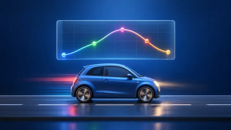
From the speed of a car you get the distance travelled: the area under the curve shows the total change.
Approximating areas with upper and lower sums and passing to the definite integral via a limit.
Fill the area under a graph with rectangles. The more rectangles, the more precisely you get the value of the integral.
Justifying the link between differentiation and integration intuitively; function and antiderivative graphically.

The area under a graph grows as you move along. Its rate of change is exactly the function itself: this is the fundamental theorem.
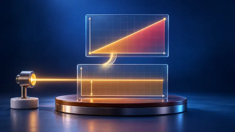
The height of one graph becomes the slope of another. If you understand bank balances, the antiderivative comes quicker than you think.
Antiderivatives of powers, eˣ, sin x and cos x; constant-factor and sum rule.
No separate simulation is planned for this.
Finding antiderivatives of functions with a linear inner function.
No separate simulation is planned for this.
Further antiderivatives by reversing the chain rule.
No separate simulation is planned for this.
Mandatory topic area. Areas between graphs, totals and mean values in context; in the advanced course also solids of revolution and improper integrals.
Calculating areas between graphs and lines parallel to the axes, also backwards (unknown bound or parameter).
No separate simulation is planned for this.
Reconstructed total, mean value and average rate of change.
From the speed of a car you get the distance travelled: the area under the curve shows the total change.
Interpreting integral expressions in context and justifying statements.
No separate simulation is planned for this.
Justifying the volume formula and calculating volumes of solids of revolution about the x-axis.
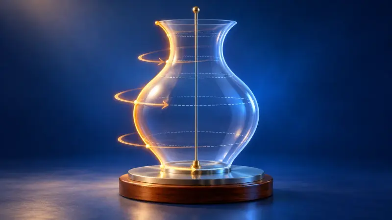
The area under a graph rotates about the x-axis and becomes a solid. Its volume is calculated with thin discs.
Examining infinitely extended regions for finite area.
No separate simulation is planned for this.
Mandatory topic area. Confident use of the introductory-phase content, combined exponential functions and growth models; in the advanced course functions with parameters and logistic growth.
Applying functions, derivatives and differentiation rules in an integrated way.
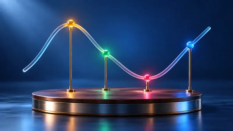
Analyse a graph step by step: zeros, maximum and minimum points, inflection points and where it rises or falls.
Investigating sums, products and compositions of exponential functions and polynomials, also in context.

Why is the number e so special? For the exponential function, the graph and its derivative are exactly the same.
Modelling exponential and bounded growth with measured data; solving exponential equations.
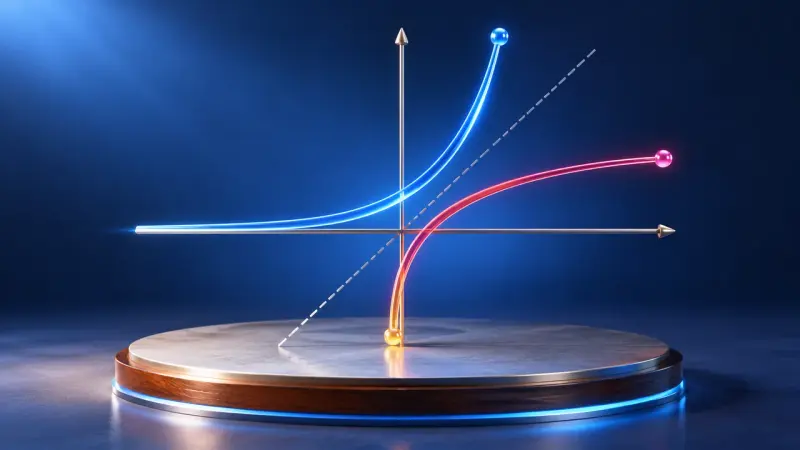
The logarithm answers the question: to what power do I raise the base to get this number? With graphs, rules and exponential equations.
Investigating the influence of parameters on combined exponential functions.

One parameter, infinitely many graphs. Where do the maxima go as k grows? Along a curve of their own, the locus.
Applying logistic growth models (without deriving them from the differential equation).
No separate simulation is planned for this.
Optional topic area. Further methods for finding antiderivatives.
Determining an antiderivative with a suitable ansatz and comparison of coefficients.
No separate simulation is planned for this.
Solving integrals of products by integration by parts.
No separate simulation is planned for this.
Simplifying integrals by substitution.
No separate simulation is planned for this.
Optional topic area. Describing growth models with differential equations and solving first-order equations.
Translating growth assumptions into differential equations.
No separate simulation is planned for this.
Slope fields, separation of variables and other elementary methods.
No separate simulation is planned for this.
Second-order differential equations, e.g. for periodic processes.
No separate simulation is planned for this.
Mandatory topic area. Further function classes (simple rational and root functions), graph transformations and inverse functions; in the advanced course the natural logarithm and compositions.
Properties and derivatives of f(x) = 1/xⁿ and f(x) = √x.
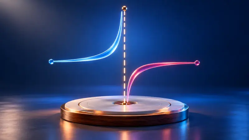
A zero or a pole, a hole or a leap to infinity? Drag the terms of the fraction and the graph shows the difference.
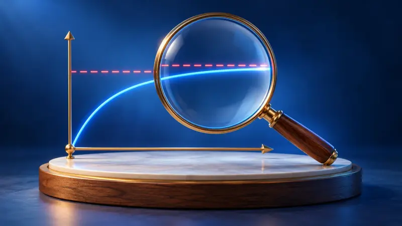
What happens to a graph when x gets very large? A point runs outwards and a magnifier shows how close it gets to the asymptote.
Shifting, stretching and reflecting graphs; interpreting g(x) = a·f(b·(x − c)) + d.
No separate simulation is planned for this.
Finding the inverse and interpreting it as reflection in y = x; domain and range.
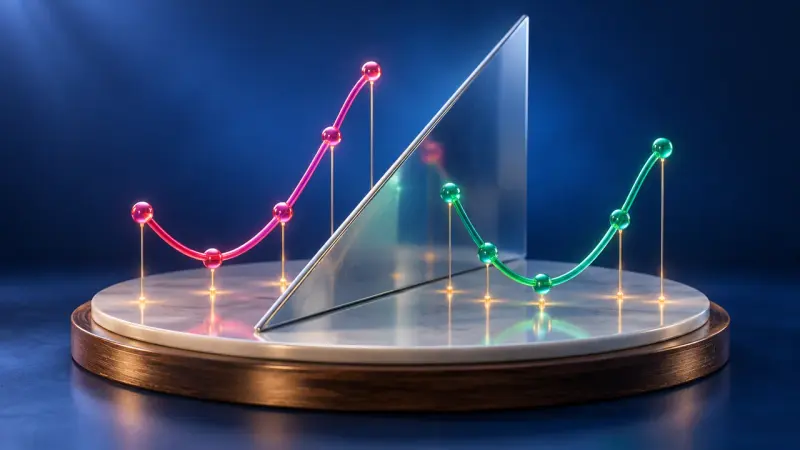
Reflect the graph in y = x and the inverse function appears. It only works if no function value occurs twice.
Describing ln as the inverse of the exponential function and transforming it.
Reflect the graph in y = x and the inverse function appears. It only works if no function value occurs twice.
The logarithm answers the question: to what power do I raise the base to get this number? With graphs, rules and exponential equations.
Using ln(x) as the antiderivative of 1/x.
No separate simulation is planned for this.
Justifying properties of sums, products and compositions from the graphs.
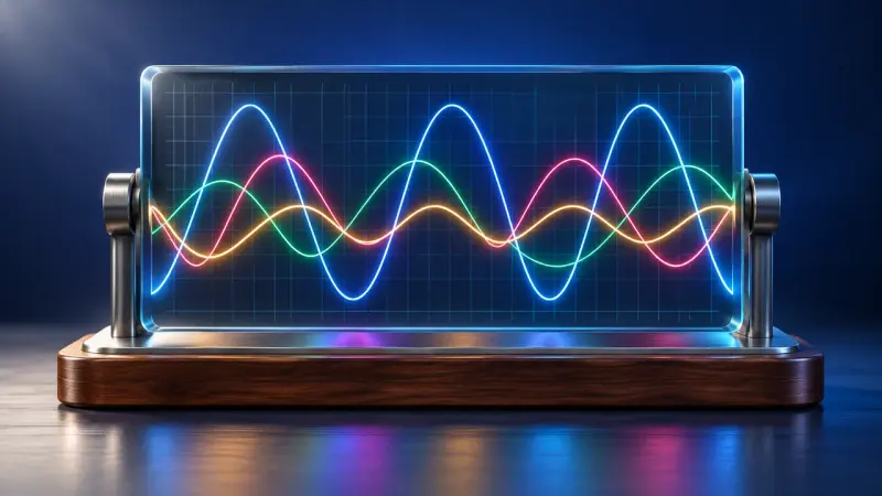
Up to three of your own functions at once, with a table of values, zeros and intersections. The tool for anything that can be a graph.
Mandatory topic area. Spatial coordinate system, vectors, dot product and angles, and investigation of simple solids and figures in space.
Representing points and solids in a 3D coordinate system, also with software.
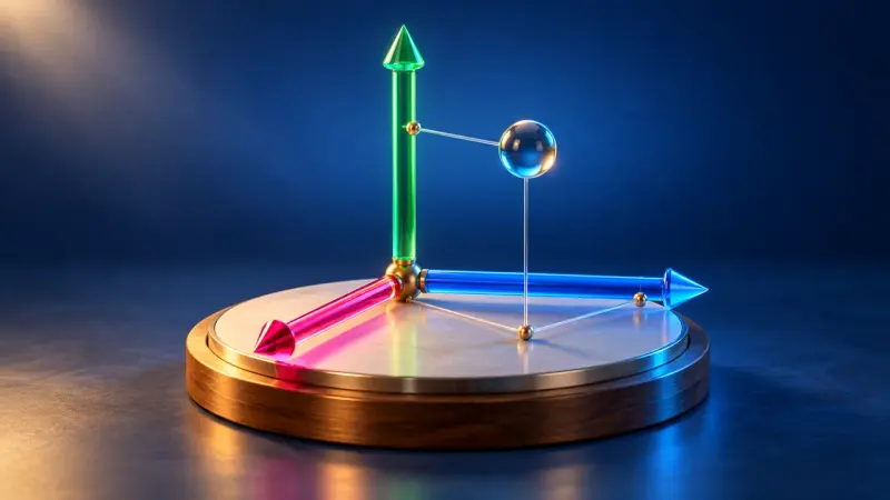
Place points in 3D coordinates, rotate the view and calculate distances with Pythagoras' theorem.
Translations as vectors, vector arithmetic, collinearity, magnitude and distance.

Drag vector arrows in space, add them and multiply them by numbers. The calculation is shown alongside in column form.
Dot product, orthogonality and angles between vectors.
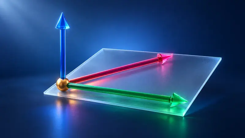
The dot product tells you the angle between two vectors; the cross product gives a perpendicular vector and an area.
Investigating and calculating cubes, prisms, pyramids and plane figures in space.
Place points in 3D coordinates, rotate the view and calculate distances with Pythagoras' theorem.
Mandatory topic area. Systems of linear equations, lines and planes in different forms, relative positions, angles, distances and applications such as shadows.
Solving systems algorithmically and interpreting solution sets geometrically.
No separate simulation is planned for this.
Lines and segments with parametric equations, point test and trace points.
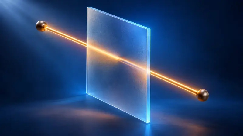
A point travels along a line through space, two vectors span a plane. Parametric, normal and coordinate forms all describe the same thing.
Intersecting, parallel, identical or skew; intersection point and angle.
A point travels along a line through space, two vectors span a plane. Parametric, normal and coordinate forms all describe the same thing.
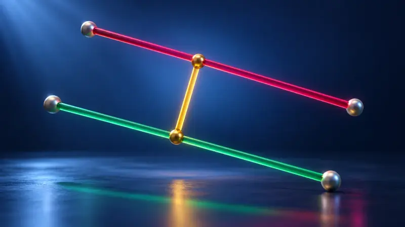
Do the lines meet, run parallel or pass each other by? In a 3D space you can turn, intersections, angles and distances become visible.
Describing motion with lines; direction vector as velocity.
A point travels along a line through space, two vectors span a plane. Parametric, normal and coordinate forms all describe the same thing.
Parametric and coordinate form, normal vector.
A point travels along a line through space, two vectors span a plane. Parametric, normal and coordinate forms all describe the same thing.
Point test and trace points of planes.
A point travels along a line through space, two vectors span a plane. Parametric, normal and coordinate forms all describe the same thing.
Converting forms; determining the position of a line relative to a plane and intersection points.
A point travels along a line through space, two vectors span a plane. Parametric, normal and coordinate forms all describe the same thing.
Do the lines meet, run parallel or pass each other by? In a 3D space you can turn, intersections, angles and distances become visible.
Intersection angles using direction and normal vectors.
No separate simulation is planned for this.
Investigating positions and angles depending on a parameter.
No separate simulation is planned for this.
Reflecting a point in a plane; foot-of-perpendicular method for point–plane distance.
Do the lines meet, run parallel or pass each other by? In a 3D space you can turn, intersections, angles and distances become visible.
Shadows, projections onto coordinate planes and area calculations.
No separate simulation is planned for this.
Describing planes via normal vector and position vector.
A point travels along a line through space, two vectors span a plane. Parametric, normal and coordinate forms all describe the same thing.
Position of two planes, lines of intersection, distances between points, lines and planes, general reflections.
Do the lines meet, run parallel or pass each other by? In a 3D space you can turn, intersections, angles and distances become visible.
Using the cross product for normal vectors and areas.
The dot product tells you the angle between two vectors; the cross product gives a perpendicular vector and an area.
Investigating lines with a parameter.
No separate simulation is planned for this.
Investigating planes with a parameter.
No separate simulation is planned for this.
Describing trajectories (e.g. of a ball) parametrically.
No separate simulation is planned for this.
Optional topic area. Modelling transition processes with graphs, state vectors and transition matrices; matrix arithmetic and Markov chains.
Modelling e.g. populations, voter movements or customer flows.
No separate simulation is planned for this.
Scalar, matrix–vector and matrix multiplication, addition, simple inverses.
No separate simulation is planned for this.
Calculating states step by step (also backwards) and finding stable states via fixed vectors.
No separate simulation is planned for this.
Interpreting entries of M² etc. in context.
No separate simulation is planned for this.
Interpreting matrix powers, limiting processes and limit matrices.
No separate simulation is planned for this.
Optional topic area. Representing and composing geometric transformations such as reflections, projections and dilations with matrices.
Describing e.g. shadows as a mapping given by a matrix.

Two arrows decide everything: wherever they point, the matrix rotates, stretches or reflects the whole grid.
Adding and multiplying matrices and finding simple inverses.
No separate simulation is planned for this.
Transformation matrices for reflections, parallel projections, central dilations and their compositions.
Two arrows decide everything: wherever they point, the matrix rotates, stretches or reflects the whole grid.
Rotations about coordinate axes, projections onto arbitrary planes through the origin, fixed points.
Two arrows decide everything: wherever they point, the matrix rotates, stretches or reflects the whole grid.
The summaries describe the curriculum in our own words. The original text is authoritative. Original text (German): Kerncurriculum, Gymnasium, Mathematics, grade 12