

Families of functions
One parameter, infinitely many graphs. Where do the maxima go as k grows? Along a curve of their own, the locus.
Qualification phase (G9: grades 12 and 13). The core curriculum has separate learning areas for the basic (gA) and the higher requirement level (eA) and does not distribute them over the years, so they are the same for the double grade 12 and 13. The codes are our own.
Turning properties into conditions on the function term, solving linear systems algorithmically and adjusting a parameter to a given property.
One parameter, infinitely many graphs. Where do the maxima go as k grows? Along a curve of their own, the locus.
Reconstructing totals from rates of change, the integral as a limit of Riemann sums, the fundamental theorem, areas bounded by graphs and antiderivatives.
Reconstructed totals, Riemann sums, the fundamental theorem and areas.

Fill the area under a graph with rectangles. The more rectangles, the more precisely you get the value of the integral.
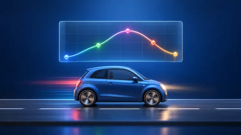
From the speed of a car you get the distance travelled: the area under the curve shows the total change.

The area under a graph grows as you move along. Its rate of change is exactly the function itself: this is the fundamental theorem.
Stating, developing and checking antiderivatives with the rules of differentiation.

The height of one graph becomes the slope of another. If you understand bank balances, the antiderivative comes quicker than you think.
The base e via (eˣ)′ = eˣ, combining and composing with other functions, product and chain rules, exponential equations and limited growth.

Why is the number e so special? For the exponential function, the graph and its derivative are exactly the same.
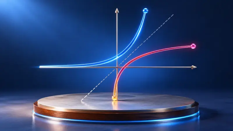
The logarithm answers the question: to what power do I raise the base to get this number? With graphs, rules and exponential equations.
Points and vectors in space, vector operations, lines and planes in parametric form, distances between points, the dot product, angles and relative positions of lines.
Points and vectors as tuples, addition and scalar multiplication, collinearity, lines and planes in parametric form.
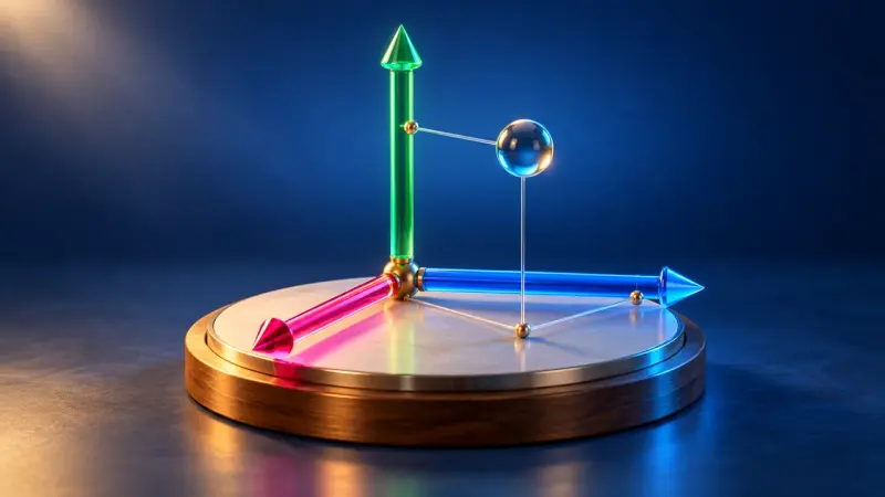
Place points in 3D coordinates, rotate the view and calculate distances with Pythagoras' theorem.

Drag vector arrows in space, add them and multiply them by numbers. The calculation is shown alongside in column form.
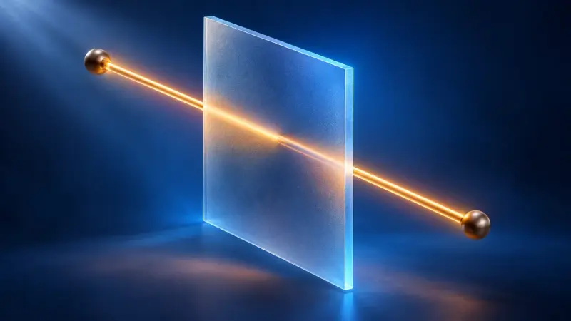
A point travels along a line through space, two vectors span a plane. Parametric, normal and coordinate forms all describe the same thing.
Distances between points, dot product and orthogonality, angles, relative positions and intersections of lines.
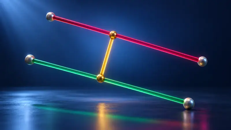
Do the lines meet, run parallel or pass each other by? In a 3D space you can turn, intersections, angles and distances become visible.
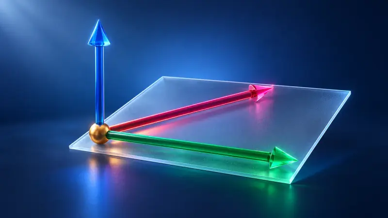
The dot product tells you the angle between two vectors; the cross product gives a perpendicular vector and an area.
Lines and planes, normal form, equations of circles and spheres.

A plane cuts the sphere in a circle, touches it at a point or misses it entirely. Including the equation of the sphere and the tangent plane.
Conditional probability and independence, expected value and standard deviation, the binomial distribution with prediction intervals and simulations.
Developing it with tree diagrams and two-way tables, checking stages for independence.

A two-way table, a Venn diagram and a tree diagram show the same data and are linked. Change one and the others follow.

A medical test is positive, but how likely is it that you are really ill? 1000 people show why the answer is often surprising.

Play yourself or simulate thousands of games: is it worth switching doors?
Calculating and interpreting measures, fair games.
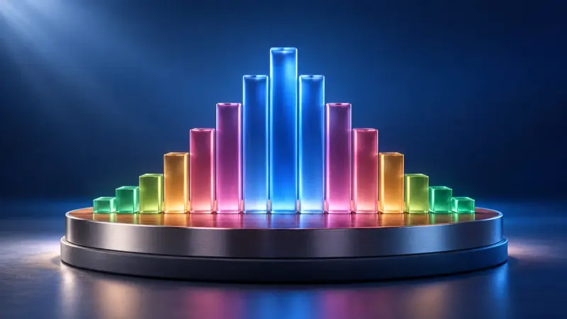
The histogram of the binomial distribution: choose a range and read off the probability directly.
Judging the model, calculating probabilities and measures, interpreting histograms, prediction intervals and whether a sample is compatible.
The histogram of the binomial distribution: choose a range and read off the probability directly.

Left or right at every pin, purely by chance. Yet every time the balls pile up into the same bell shape.
As at basic level, plus the integral function, ln as an antiderivative of 1/x, solids of revolution and improper integrals.
Reconstructed totals, Riemann sums, the fundamental theorem and areas.
Fill the area under a graph with rectangles. The more rectangles, the more precisely you get the value of the integral.
From the speed of a car you get the distance travelled: the area under the curve shows the total change.
The area under a graph grows as you move along. Its rate of change is exactly the function itself: this is the fundamental theorem.
The integral function as accumulation or area function, antiderivatives including ln.
The height of one graph becomes the slope of another. If you understand bank balances, the antiderivative comes quicker than you think.
The area under a graph grows as you move along. Its rate of change is exactly the function itself: this is the fundamental theorem.
Volumes of solids of revolution about the x-axis, improper integrals.
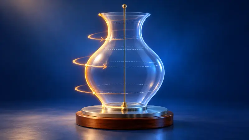
The area under a graph rotates about the x-axis and becomes a solid. Its volume is calculated with thin discs.
Comparing limited and logistic growth, differential equations as models, the exponential function with its derivative, combinations and compositions, and exponential equations.
Limited and logistic growth, asymptotic behaviour, differential equations.
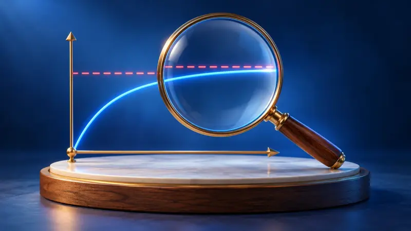
What happens to a graph when x gets very large? A point runs outwards and a magnifier shows how close it gets to the asymptote.
The base e, derivatives, product and chain rules, exponential equations and family parameters.
Why is the number e so special? For the exponential function, the graph and its derivative are exactly the same.
The logarithm answers the question: to what power do I raise the base to get this number? With graphs, rules and exponential equations.
As at basic level, plus projection onto the plane with matrices, planes in normal and coordinate form, distances between points, lines and planes, and Gaussian elimination.
Points and vectors, vector operations, collinearity and oblique drawings with projection matrices.
Place points in 3D coordinates, rotate the view and calculate distances with Pythagoras' theorem.
Drag vector arrows in space, add them and multiply them by numbers. The calculation is shown alongside in column form.
Lines and planes in parametric, normal and coordinate form.
A point travels along a line through space, two vectors span a plane. Parametric, normal and coordinate forms all describe the same thing.
Distances, dot product, angles, relative positions of lines and planes, and Gaussian elimination.
Do the lines meet, run parallel or pass each other by? In a 3D space you can turn, intersections, angles and distances become visible.
The dot product tells you the angle between two vectors; the cross product gives a perpendicular vector and an area.
Vectors in other contexts, further transformation matrices, equations of circles and spheres.

Two arrows decide everything: wherever they point, the matrix rotates, stretches or reflects the whole grid.
A plane cuts the sphere in a circle, touches it at a point or misses it entirely. Including the equation of the sphere and the tangent plane.
Classifying functions by global properties and fitting them to data, piecewise functions, and families of polynomial and exponential functions.
Using symmetry, behaviour for large |x|, asymptotes and periodicity, setting up conditions, continuity and differentiability.
What happens to a graph when x gets very large? A point runs outwards and a magnifier shows how close it gets to the asymptote.
The effect of the family parameter and fitting to properties.
One parameter, infinitely many graphs. Where do the maxima go as k grows? Along a curve of their own, the locus.
As at basic level, plus causal and stochastic independence, the normal distribution, approximating the binomial distribution and confidence intervals.
Tree diagrams and two-way tables, causal and stochastic independence.
A two-way table, a Venn diagram and a tree diagram show the same data and are linked. Change one and the others follow.
A medical test is positive, but how likely is it that you are really ill? 1000 people show why the answer is often surprising.
Play yourself or simulate thousands of games: is it worth switching doors?
Calculating and interpreting measures, fair games.
The histogram of the binomial distribution: choose a range and read off the probability directly.
The model, probabilities, measures, histograms, prediction intervals and simulations.
The histogram of the binomial distribution: choose a range and read off the probability directly.
Left or right at every pin, purely by chance. Yet every time the balls pile up into the same bell shape.
Discrete and continuous random variables, parameters of the normal distribution.
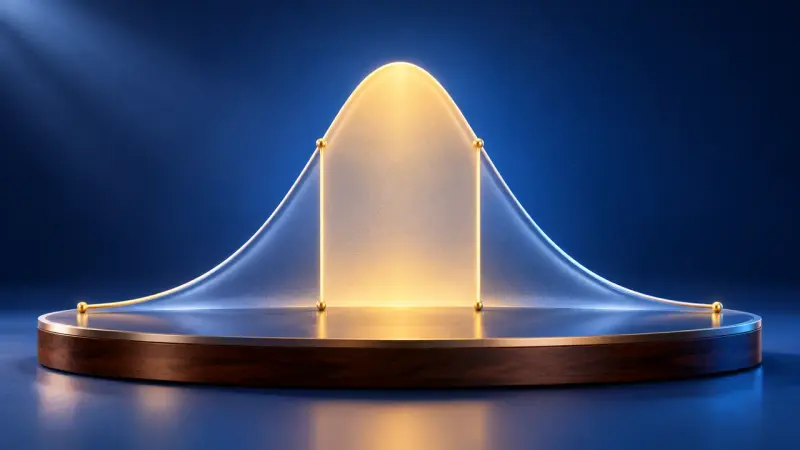
How many bottles are underfilled? Under the bell curve every probability is an area, with the sigma rules as a rule of thumb.
Approximating the binomial distribution, sigma intervals and confidence intervals.
How many bottles are underfilled? Under the bell curve every probability is an area, with the sigma rules as a rule of thumb.
Left or right at every pin, purely by chance. Yet every time the balls pile up into the same bell shape.
The summaries describe the curriculum in our own words. The original text is authoritative. Original text (German): Kerncurriculum, Gymnasium, Mathematics, grade 12/13