
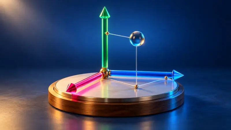
Points and solids in 3D coordinates
Place points in 3D coordinates, rotate the view and calculate distances with Pythagoras' theorem.
Qualification phase, third and fourth half-year (Q3, Q4; at the Gymnasium with Abitur after grade 12: grade 12). Q4 also deepens and links all three areas. LK = advanced course only. The numbers are our own.
Coordinates, vectors, the dot product, lines and planes with relative positions, angles and distances.
Describing geometry with coordinates, calculating with vectors, testing for collinearity and using the dot product for lengths and angles.
Place points in 3D coordinates, rotate the view and calculate distances with Pythagoras' theorem.

Drag vector arrows in space, add them and multiply them by numbers. The calculation is shown alongside in column form.
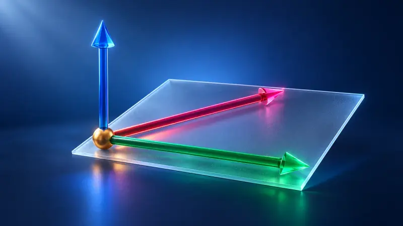
The dot product tells you the angle between two vectors; the cross product gives a perpendicular vector and an area.
Lines and planes in parametric, coordinate and normal form, relative positions and distances; LK: also families and distances point–line and line–line.
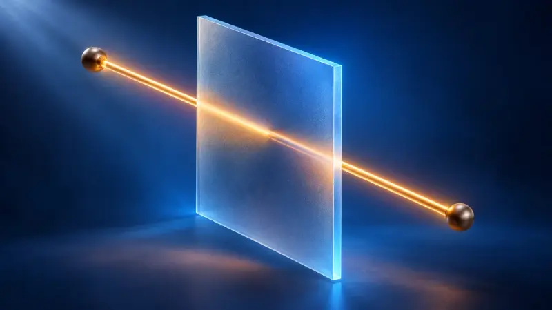
A point travels along a line through space, two vectors span a plane. Parametric, normal and coordinate forms all describe the same thing.
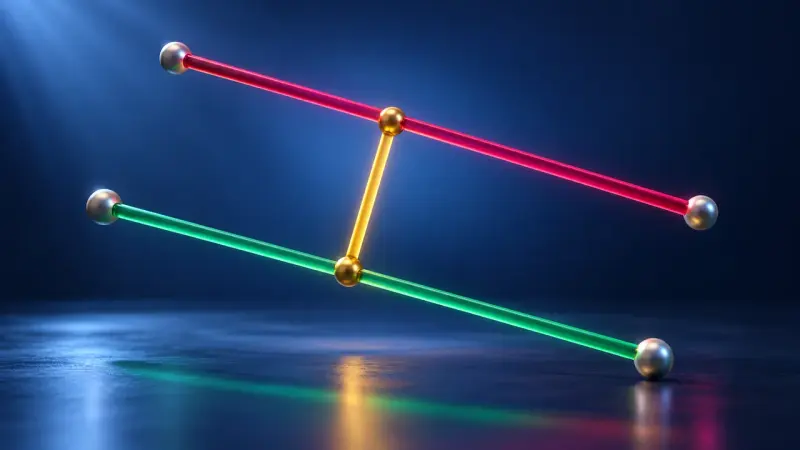
Do the lines meet, run parallel or pass each other by? In a 3D space you can turn, intersections, angles and distances become visible.
The binomial distribution with its parameters, inferring from the sample to the population, hypothesis tests (LK) and the normal distribution (LK), and further calculus.
Deepening and linking differential and integral calculus; LK: solids of revolution and improper integrals.

Which box holds the most, which can uses the least metal? Five everyday problems show how to find the best solution with the derivative.
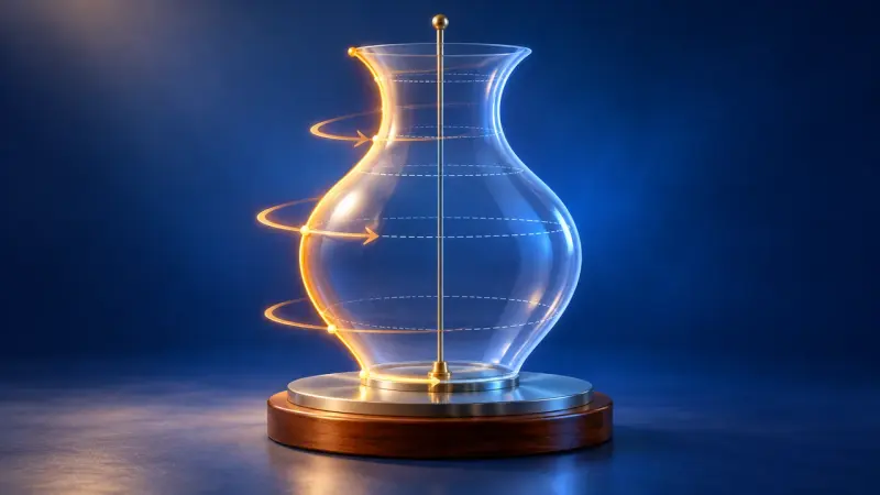
The area under a graph rotates about the x-axis and becomes a solid. Its volume is calculated with thin discs.

One parameter, infinitely many graphs. Where do the maxima go as k grows? Along a curve of their own, the locus.

The area under a graph grows as you move along. Its rate of change is exactly the function itself: this is the fundamental theorem.
The binomial distribution with expected value and standard deviation, k-σ intervals and significance; LK: hypothesis tests with type I and type II errors, the bell shape of the normal distribution.

Left or right at every pin, purely by chance. Yet every time the balls pile up into the same bell shape.

The histogram of the binomial distribution: choose a range and read off the probability directly.
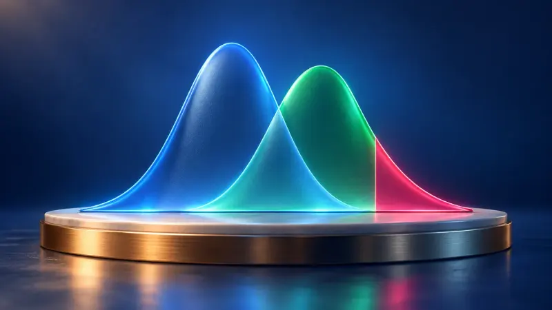
A test decides between two hypotheses. Coloured areas show how often it can be wrong.
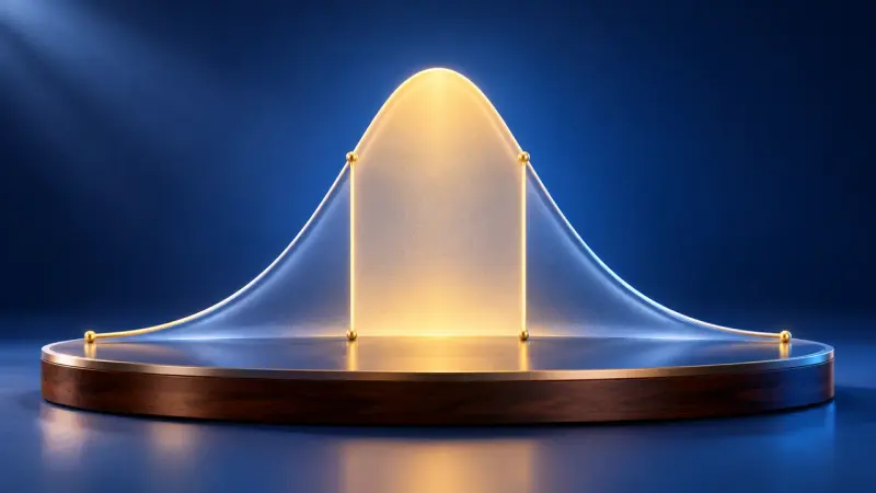
How many bottles are underfilled? Under the bell curve every probability is an area, with the sigma rules as a rule of thumb.
Tasks that link calculus, analytic geometry and probability.
No separate simulation is planned for this.
Possible additional courses: non-Euclidean geometry, logic, number theory, numerical mathematics, differential equations, sequences and series with Taylor series, Markov chains, complex analysis, conic sections, further calculus, reasoning and proof.

Term by term a polynomial hugs a function such as sin x ever more closely. That is pretty much how a calculator does it.
The summaries describe the curriculum in our own words. The original text is authoritative. Original text (German): Rahmenlehrplan, Gymnasium, Mathematics, grade 12