

Newton’s method
Approximate a zero with tangent lines. Each step gets you closer, but sometimes it goes wrong.
Course phase (grades 12/13); the same content is also listed under grade 13. Advanced course (3.5, headings marked “(advanced course only)”) and basic course (3.6, “(basic course)”) are combined in this entry.
Approximating e and zeros, product and chain rules, rules of integration and improper integrals; scalar and vector product and Gaussian elimination for linear systems.
Approximating Euler’s number and justifying and carrying out an iterative method for zeros.
Approximate a zero with tangent lines. Each step gets you closer, but sometimes it goes wrong.

Term by term a polynomial hugs a function such as sin x ever more closely. That is pretty much how a calculator does it.
Applying the product and chain rules, also for simple rational functions.
No separate simulation is planned for this.
Finding antiderivatives with the power, constant-factor and sum rules and linear substitution, calculating definite integrals with the fundamental theorem and investigating improper integrals.

The area under a graph grows as you move along. Its rate of change is exactly the function itself: this is the fundamental theorem.
Calculating, interpreting geometrically and using the scalar and vector product.

The dot product tells you the angle between two vectors; the cross product gives a perpendicular vector and an area.
Explaining Gaussian elimination as an algorithm, carrying it out also in matrix notation and interpreting the solution set of a 3×3 system geometrically.

Two arrows decide everything: wherever they point, the matrix rotates, stretches or reflects the whole grid.
Angles, distances (also between skew lines) and areas using scalar and vector products; the integral for areas, mean values and volumes of revolution.
Orthogonality and angles with the scalar product, angles between lines and planes, distances using the Hessian normal form and between skew lines, and areas with the vector product.
The dot product tells you the angle between two vectors; the cross product gives a perpendicular vector and an area.

Do the lines meet, run parallel or pass each other by? In a 3D space you can turn, intersections, angles and distances become visible.
Interpreting the integral as a limit of sums, calculating mean values of functions, areas between graphs and volumes of solids of revolution.

Fill the area under a graph with rectangles. The more rectangles, the more precisely you get the value of the integral.

The area under a graph rotates about the x-axis and becomes a solid. Its volume is calculated with thin discs.
Planes in parametric, coordinate and normal form and relative positions in space; reflections, motions and proofs with vectors.
Interpreting scalar and vector product geometrically and finding a vector perpendicular to two given ones.
The dot product tells you the angle between two vectors; the cross product gives a perpendicular vector and an area.
Showing planes with trace lines, describing them in three forms and converting between them, determining relative positions and intersections, and handling reflections, distances, areas, volumes and straight-line motion.
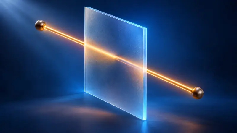
A point travels along a line through space, two vectors span a plane. Parametric, normal and coordinate forms all describe the same thing.
Do the lines meet, run parallel or pass each other by? In a 3D space you can turn, intersections, angles and distances become visible.

A plane cuts the sphere in a circle, touches it at a point or misses it entirely. Including the equation of the sphere and the tangent plane.
Proving simple geometric theorems with vectors.
No separate simulation is planned for this.
Natural exponential and logarithmic functions, inverse and composite functions; optimisation problems, finding functions from properties and families of functions; the integral, the fundamental theorem and reconstructing quantities.
Explaining the role of base e, sketching the graphs of eˣ and ln x as inverse functions and stating their derivatives and an antiderivative of eˣ.

Why is the number e so special? For the exponential function, the graph and its derivative are exactly the same.
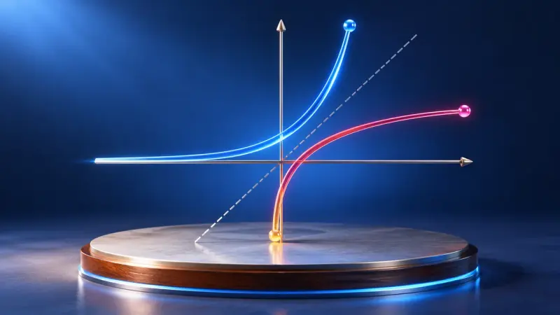
The logarithm answers the question: to what power do I raise the base to get this number? With graphs, rules and exponential equations.
Determining domains and ranges, proving invertibility via strict monotonicity and finding terms of inverse functions.

Reflect the graph in y = x and the inverse function appears. It only works if no function value occurs twice.
Forming and recognising compositions, investigating quotients of known functions for asymptotes and zeros, and analysing sums, products and compositions.

A zero or a pole, a hole or a leap to infinity? Drag the terms of the fraction and the graph shows the difference.

Up to three of your own functions at once, with a table of values, zeros and intersections. The tool for anything that can be a graph.

What happens to a graph when x gets very large? A point runs outwards and a magnifier shows how close it gets to the asymptote.

Square, sawtooth and other waves are built from many sine waves. You can also listen to them.
Solving optimisation problems with constraints, finding function terms from given properties and investigating families of functions.

One parameter, infinitely many graphs. Where do the maxima go as k grows? Along a curve of their own, the locus.

Which box holds the most, which can uses the least metal? Five everyday problems show how to find the best solution with the derivative.
Interpreting the integral as signed area and change of a quantity, reconstructing quantities from rates of change, distinguishing and using the fundamental theorem, integral function and antiderivative, and reasoning graphically between a function and its antiderivative.
The area under a graph grows as you move along. Its rate of change is exactly the function itself: this is the fundamental theorem.

The height of one graph becomes the slope of another. If you understand bank balances, the antiderivative comes quicker than you think.
Fill the area under a graph with rectangles. The more rectangles, the more precisely you get the value of the integral.

From the speed of a car you get the distance travelled: the area under the curve shows the total change.
One- and two-sided hypothesis tests for binomially distributed random variables with type I and type II errors; the normal distribution as a continuous distribution.
Explaining the logic of testing, formulating null hypotheses, determining and showing rejection region and significance, and explaining type I and type II errors and the influence of sample size.
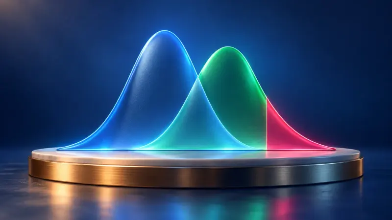
A test decides between two hypotheses. Coloured areas show how often it can be wrong.

The histogram of the binomial distribution: choose a range and read off the probability directly.
Distinguishing discrete and continuous random variables, stating the density function with mean and standard deviation, and calculating probabilities for approximately normally distributed variables.

Left or right at every pin, purely by chance. Yet every time the balls pile up into the same bell shape.

How many bottles are underfilled? Under the bell curve every probability is an area, with the sigma rules as a rule of thumb.
Natural logarithm, product rule and chain rule with a linear inner function, rules of integration; scalar and vector product and Gaussian elimination without parameters.
Solving exponential equations with the natural logarithm.
The logarithm answers the question: to what power do I raise the base to get this number? With graphs, rules and exponential equations.
Applying the product rule and the chain rule (with a linear inner function).
No separate simulation is planned for this.
Finding antiderivatives with the basic rules and linear substitution and calculating definite integrals with the fundamental theorem.
The area under a graph grows as you move along. Its rate of change is exactly the function itself: this is the fundamental theorem.
Calculating the scalar and vector product and using them in calculations.
The dot product tells you the angle between two vectors; the cross product gives a perpendicular vector and an area.
Applying Gaussian elimination up to row echelon form and stating the number of solutions.
No separate simulation is planned for this.
Angles, the distance between a point and a plane and areas using scalar and vector products; the integral for calculating areas.
Checking orthogonality and angles with the scalar product, finding angles of intersection and the distance from a point to a plane, and calculating areas with the vector product.
The dot product tells you the angle between two vectors; the cross product gives a perpendicular vector and an area.
Do the lines meet, run parallel or pass each other by? In a 3D space you can turn, intersections, angles and distances become visible.
Describing the integral intuitively as a limiting process and finding areas between a graph and the x-axis and between two graphs.
Fill the area under a graph with rectangles. The more rectangles, the more precisely you get the value of the integral.
Planes in parametric and coordinate form and the relative position of line and plane and of two planes; applications such as reflections and straight-line motion.
Interpreting scalar and vector product geometrically and finding a common perpendicular vector.
The dot product tells you the angle between two vectors; the cross product gives a perpendicular vector and an area.
Showing planes with trace lines, describing them in parametric and coordinate form, investigating line–plane and plane–plane positions and solving applied problems.
A point travels along a line through space, two vectors span a plane. Parametric, normal and coordinate forms all describe the same thing.
Do the lines meet, run parallel or pass each other by? In a 3D space you can turn, intersections, angles and distances become visible.
The natural exponential function and simple composite functions; extrema in real contexts and finding functions; the integral as area and change of a quantity, the fundamental theorem.
Describing the special base e, sketching the graph of eˣ with its asymptote and stating its derivative and antiderivative.
Why is the number e so special? For the exponential function, the graph and its derivative are exactly the same.
Recognising compositions with a linear inner function and investigating sums, products and such compositions.
Up to three of your own functions at once, with a table of values, zeros and intersections. The tool for anything that can be a graph.
Finding extrema in real contexts and determining uniquely defined function terms.
Which box holds the most, which can uses the least metal? Five everyday problems show how to find the best solution with the derivative.
Interpreting the integral as signed area and change of a quantity, reconstructing quantities, applying the fundamental theorem and reasoning graphically between a function and its antiderivative.
The area under a graph grows as you move along. Its rate of change is exactly the function itself: this is the fundamental theorem.
The height of one graph becomes the slope of another. If you understand bank balances, the antiderivative comes quicker than you think.
From the speed of a car you get the distance travelled: the area under the curve shows the total change.
From the binomial to the normal distribution: discrete and continuous random variables and the bell curve.
Distinguishing discrete and continuous random variables, describing how mean and standard deviation shape the bell curve, and calculating probabilities.
Left or right at every pin, purely by chance. Yet every time the balls pile up into the same bell shape.
How many bottles are underfilled? Under the bell curve every probability is an area, with the sigma rules as a rule of thumb.
The summaries describe the curriculum in our own words. The original text is authoritative. Original text (German): Bildungsplan, Gymnasium, Mathematics, grade 12/13