
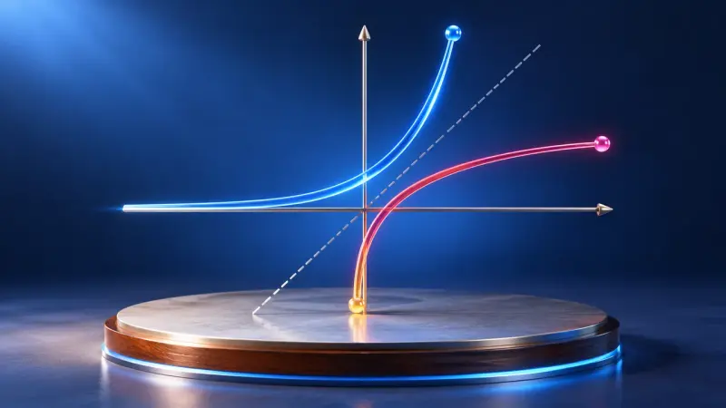
Logarithms as the inverse of exponentiation
The logarithm answers the question: to what power do I raise the base to get this number? With graphs, rules and exponential equations.
Studienstufe, second year (S3/S4; at the Gymnasium: grade 12): modules 4 and 5 and one of the elective modules 6 (analytic geometry) and 7 (linear algebra). eA = higher level only. The numbers are the module numbers of the curriculum.
Growth models with exponential functions, Euler’s number, the ln function as the inverse, derivatives and integrals as changes in totals; eA: families of functions, finding zeros numerically.
The logarithm answers the question: to what power do I raise the base to get this number? With graphs, rules and exponential equations.

Reflect the graph in y = x and the inverse function appears. It only works if no function value occurs twice.

Why is the number e so special? For the exponential function, the graph and its derivative are exactly the same.

Approximate a zero with tangent lines. Each step gets you closer, but sometimes it goes wrong.

Analyse a graph step by step: zeros, maximum and minimum points, inflection points and where it rises or falls.

One parameter, infinitely many graphs. Where do the maxima go as k grows? Along a curve of their own, the locus.

From the speed of a car you get the distance travelled: the area under the curve shows the total change.
Discrete random variables, the binomial distribution with expected value, standard deviation and sigma rules; eA: hypothesis tests and the normal distribution.

Left or right at every pin, purely by chance. Yet every time the balls pile up into the same bell shape.

The histogram of the binomial distribution: choose a range and read off the probability directly.
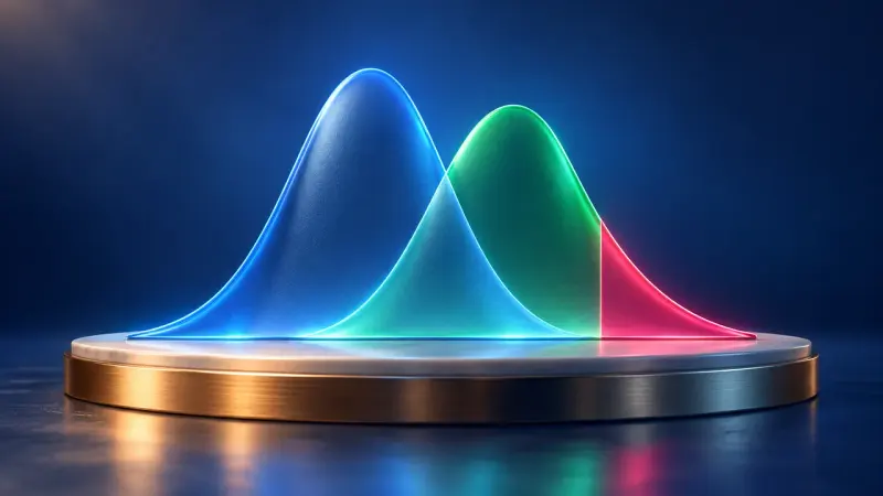
A test decides between two hypotheses. Coloured areas show how often it can be wrong.

How many bottles are underfilled? Under the bell curve every probability is an area, with the sigma rules as a rule of thumb.
Lines and planes with vectors, plane equations, trace points, relative positions, intersections and angles, normal vectors, reflection; eA: distances, Gaussian elimination.

The dot product tells you the angle between two vectors; the cross product gives a perpendicular vector and an area.

A point travels along a line through space, two vectors span a plane. Parametric, normal and coordinate forms all describe the same thing.

Do the lines meet, run parallel or pass each other by? In a 3D space you can turn, intersections, angles and distances become visible.
Systems of linear equations with Gaussian elimination, growth and redistribution processes with transition matrices, matrix powers, fixed vectors and long-term behaviour.
No separate simulation is planned for this.
The summaries describe the curriculum in our own words. The original text is authoritative. Original text (German): Bildungsplan, Gymnasium, Mathematics, grade 12